
NAM A2: THE COMPLETE GUIDE
Everything you need to know about Neural Amp Modeler (NAM) Architecture 2 (A2): how it sounds, how it works, and how to use it.
In this guide
Welcome to the definitive guide on NAM Architecture 2 (A2), the next generation of Neural Amp Modeler. This open-source technology lets anyone capture and share hyper-realistic digital models (technically “neural models”) of amplifiers, guitar and bass pedals, outboard gear, and full signal chains.
A2 is the result of a six-month partnership between TONE3000 and Steve Atkinson, the creator of NAM. The goals were to improve overall accuracy and increase efficiency, so that NAM could run natively on the small chips found in mass-market embedded hardware, like budget multi-fx pedals. In our tests, we found that A2 is the most accurate amp modeling technology ever built, and it's efficient enough to run on a $3 chip.
If you're new to NAM, start with our guide on Neural Amp Modeler first, then come back here.
The Basics
What is NAM Architecture 2 (A2)?
A2 is the next generation of Neural Amp Modeler. It was built from the ground up by TONE3000 in partnership with Steve Atkinson, the creator of NAM, and it replaces the original architecture, called Architecture 1 (A1), as the default for all new captures on TONE3000. According to our tests below, A2 is the most accurate amp modeling technology.
How do I play through A2 models?
- Browse and download A2 tones via TONE3000: tone3000.com/search
- Download the latest NAM plugin "Gateway": neuralampmodeler.com/users
- Choose
Select model directory...and select your downloaded A2 tones
Can I still find A1 models on TONE3000?
Yes. You can access all legacy A1 models on TONE3000. Here's how:
1. Visit https://www.tone3000.com/search
2. Filters > Technical > choose "A1 – Legacy"
3. On the tone pack page, scroll down to "Models" and select "A1 Legacy"
4. Click "Download all A1"
What if my hardware or software doesn't support A2?
The fastest way to get A2 (and the TONE3000 API) into your gear is to ask the company directly. The more players who request it, the faster it gets prioritized. Here's a message you can edit and send to any manufacturer below.
Is A2 one NAM model?
Yes. An A2 download is a single NAM model that can be run as either A2-Full or A2-Lite.
What are A2-Full and A2-Lite?
A2-Full is the maximum-accuracy version, built for pro-audio contexts like DAWs and devices with sufficient processing headroom.
A2-Lite is the same model run at a smaller size, designed for processing-constrained devices like multi-fx pedals and mini amps. Even at the smaller size, A2-Lite still beats every other commercial modeler we tested. A2-Lite is what makes native NAM support possible on commercial embedded hardware.
How do A2-Full and A2-Lite sound?
In our quantitative tests and blind listening tests, A2-Full beat Neural DSP V2 and V1, IK Multimedia’s ToneX V2, and Line 6’s Proxy by a wide margin. It also improves on A1-Standard, the previous NAM architecture, while running at a lower CPU cost. A2-Lite also beat all of these commercial modelers. In blind listening tests it scores right alongside A1-Standard, despite running in a fraction of the CPU budget.
Amp Modeler Blind Listening Test
Over 1,000 participants compared recordings of real gear to anonymized digital models using the MUSHRA blind listening methodology. Higher scores mean the model was rated as sounding closer to the original amp, pedal, or signal chain.
Amp Modeler Accuracy Test
Each model's output was compared against recordings of real gear using several error metrics (ESR, MAE, LOG_MEL, and MRSTFT). This chart shows Bayesian Elo ratings derived from ESR, where higher scores indicate lower measured error relative to the original amp, pedal, or signal chain.
Tests were conducted in March 2026 using the latest modelers from Neural DSP, IK Multimedia ToneX, and Line 6 Proxy.
You can learn more about our tests in The Technical Deep Dive section.
How efficient are A2-Full and A2-Lite?
A2-Full is roughly 30–40% more performant than A1-Standard. You can run three A2-Full models for the same CPU cost as two A1-Standard models, with better accuracy. To put that in perspective, a MacBook with an Apple M-series chip can run 64 A2-Full models at once.
A2-Lite runs at 50% CPU on an ARM Cortex M7 600MHz which costs $3 per unit when sold in bulk. That's the same chip class behind today's mass-market gear, found in pedals like the IK Multimedia ToneX One. This dramatic improvement in efficiency makes NAM possible on mass-market hardware for the first time. An M-series MacBook can run ~200 A2-Lite models at once.
A1 vs A2 Inference Speed
How the new A2 models compare to the original A1 architecture on the same hardware.
For the engineering behind these numbers, see How does A2 run so efficiently?.
Is A2 open source?
Yes. A2 is fully MIT-licensed. The code is on GitHub, free to use, modify, and ship in commercial products with no license fees.
- C++ inference engine: github.com/sdatkinson/NeuralAmpModelerCore
- Trainer: github.com/sdatkinson/neural-amp-modeler
- Official demo plugin: github.com/sdatkinson/NeuralAmpModelerPlugin
- TONE3000 embedded data loader: github.com/tone-3000/nam-binary-loader
- TONE3000 embedded pure-C guide: github.com/tone-3000/nam-pedal
- TONE3000 WASM engine: github.com/tone-3000/neural-amp-modeler-wasm
What about A2-Nano?
A2-Nano was the original name for A2-Lite, used in early blog posts and partner emails before the official launch. We ultimately renamed it to avoid confusion with the existing A1-Nano model. If you see "A2-Nano" referenced anywhere, it means A2-Lite :)
Can A2 capture more types of gear?
Yes. Our quantitative and listening tests spanned a wide range of gear such as guitar and bass amps, amp and cab rigs, pedals, and outboard gear like channel strips. We deliberately stress-tested the edges with historically tricky devices like octave fuzz pedals.
A2 can capture more types of gear, in part because it has a larger "receptive field," around 50 percent longer. In plain terms, the model takes in a longer window of recent signal before predicting the response, a kind of short-term memory for what just happened. That longer window lets it model more time-dependent behavior, like sag and compression. The practical payoff is twofold: more of what makes real gear feel alive and responsive comes through, and gear that depends heavily on timing, for example compressors at reasonable attack and release settings, can now be captured faithfully.
Who built A2?
A2 was built by TONE3000's Woodbury Shortridge (Co-Founder and CTO) and João Felipe Santos, PhD (ML and embedded engineer), in partnership with the creator of NAM, Steve Atkinson, PhD.
The Basics cont.
Can I expect lower ESRs with A2 compared to A1?
Yes, across the board. When TONE3000 retrained the full library to A2, we compared each model's A2 accuracy against its A1 accuracy, and A2 captures consistently produce lower ESR values. This means A2 models match the real gear more closely sample by sample than A1 models.
The chart below shows the ESR distribution between A1 and A2 models (lower is better). The median ESR roughly halved, from 0.0062 with A1-Standard to 0.0033 with A2-Full.
A2 vs A1 Accuracy
We retrained the entire library of A1 models with A2 and compared the resulting ESR against the original A1 captures (lower is better).
Does A2 handle artifacts like aliasing better than A1?
Yes. Historically, small WaveNet-based models can introduce two kinds of artifacts that aren't present in real gear. The first are aliasing-like artifacts, which are inharmonic frequencies that appear when you play high-frequency content. The second are "ring" artifacts, which can be heard as metallic ringing that’s especially noticeable on models of high gain amps. A2 significantly reduced both. The How does A2 reduce high-frequency artifacts? section below covers this topic in more detail.
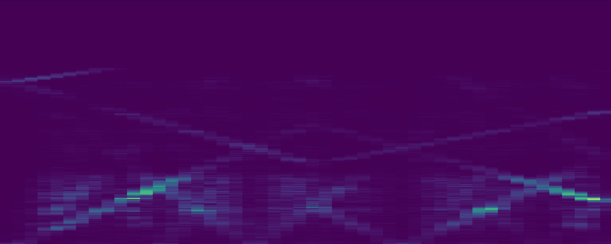
Aliasing-like Artifacts
The same sine sweep run through the old and new model designs, compared against the recording.


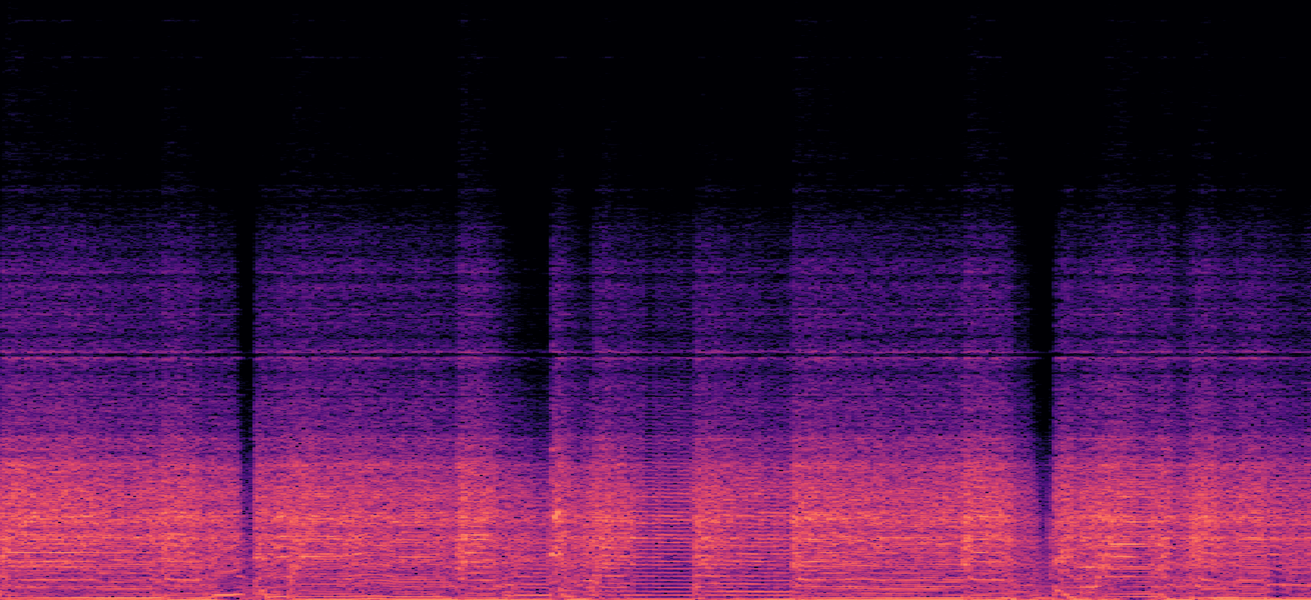
Spectral Ring Artifacts
White noise bursts run through each model variant. Pay attention to the ringing artifact around 10 kHz.
How does A2-Full compare to custom architectures like xSTD, hyper-accuracy, and REVyHI?
A2 often has comparable accuracy, is faster to train, and requires less CPU. We love these community-built architectures, and we studied them as part of the development of A2. They are amazingly accurate, but they take hours to train and require much more CPU than A1.
Our goal with A2 was to give the community the accuracy they were seeking while also increasing efficiency, so that these models could run on mass market hardware. We’re grateful for the community’s contributions – A2 wouldn’t be possible without them.
How does NAM A2 compare to Neural DSP Quad Cortex, IK Multimedia ToneX, and Line 6 Proxy?
A2 beats them in qualitative and blind listening tests. Charts below.
Amp Modeler Blind Listening Test
Over 1,000 participants compared recordings of real gear to anonymized digital models using the MUSHRA blind listening methodology. Higher scores mean the model was rated as sounding closer to the original amp, pedal, or signal chain.
Amp Modeler Accuracy Test
Each model's output was compared against recordings of real gear using several error metrics (ESR, MAE, LOG_MEL, and MRSTFT). This chart shows Bayesian Elo ratings derived from ESR, where higher scores indicate lower measured error relative to the original amp, pedal, or signal chain.
Tests were conducted in March 2026 using the latest modelers from Neural DSP, IK Multimedia ToneX, and Line 6 Proxy.
How is NAM A2 different from other commercial modelers?
NAM A2 is open source. Commercial amp modelers, including Neural DSP Quad Cortex, IK Multimedia ToneX, Line 6 Helix, and others, are proprietary closed-source systems. That means the tones you create or use in their products can only be used with their hardware or software.
A2 works differently. It is an open protocol for tone, similar to IR or MIDI files. Tones created with NAM A2 work anywhere NAM is supported, including a growing ecosystem of plugins, multi-fx pedals, amps, and other products.
Because A2 is fully open source, the model architecture, training code, and inference engine are free to use, modify, and ship in commercial products. Each developer who builds with NAM can contribute to our global community and advance the technology for everyone.
With the TONE3000 API, hardware and software makers can also bring TONE3000’s massive library of NAM A2 captures and impulse responses directly into their products.
Migration and Compatibility
Do I need to retrain my models to A2?
No. TONE3000 has already retrained the full library of existing A1 models. The only exceptions were models with zero downloads that were more than 60 days old, and models with malformed training data. Those remain available as A1 models, and creators can retrain them manually if needed. If you think your models weren't retrained by mistake, reach out to us at support@tone3000.com.
How did TONE3000 retrain from A1 to A2?
TONE3000 retrained models to A2 in two ways, depending on whether we had access to the original training data.
- If you trained your NAM captures on TONE3000, we had your original training data: the original recording of your gear. We used that data to train new A2 models that sound significantly better than A1, confirmed by both our blind listening tests and quantitative tests.
- If you did not train your NAM captures on TONE3000, we generated synthetic training data from your A1 models to train new A2 models. These models sound as good as A1 but run far more efficiently: A2-Full uses 30 to 40% less CPU, and A2-Lite uses dramatically less. They're also compatible with the new ecosystem, so they run on all hardware and software that supports A2. You'll see these labeled as "Convert" in the Models section of the tone pack page.
Is A2 backwards compatible?
No. A2 is a new architecture, not a drop-in update. Hardware and software companies that previously supported A1 will need to update their integrations to support A2. Most major partners are doing this now, and we expect broad A2 support across the NAM ecosystem by the end of 2026.
Will my A1 captures still work?
Yes. You can still upload A1 models to TONE3000 and run them in hardware and software that supports A1. That said, TONE3000 is significantly deprioritizing A1 in favor of A2. If you're creating a new capture today, you should train it as A2.
How are A2 captures differentiated from A1 when browsing TONE3000?
Every tone retrained to A2 carries an "A2" badge on the tone pack page. You can also filter by architecture from the browse and search views.
Can I still train A1 or custom architectures on TONE3000?
No. The default training pipeline now only supports A2. We plan to launch a training playground that supports new custom architecture options for advanced users and researchers later this year.
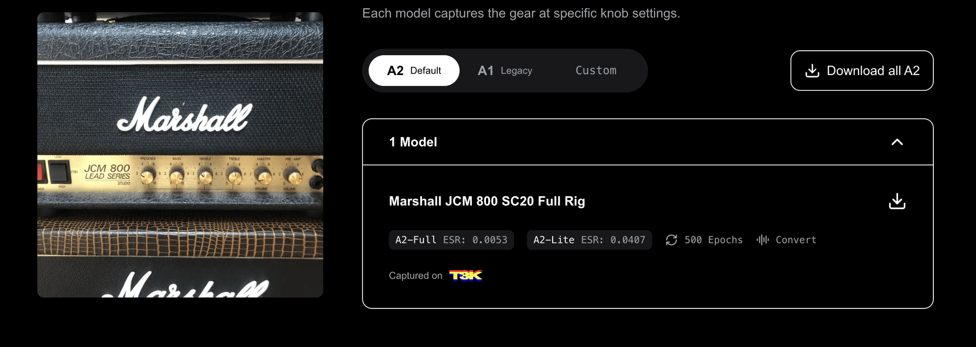
How do I capture my gear with A2?
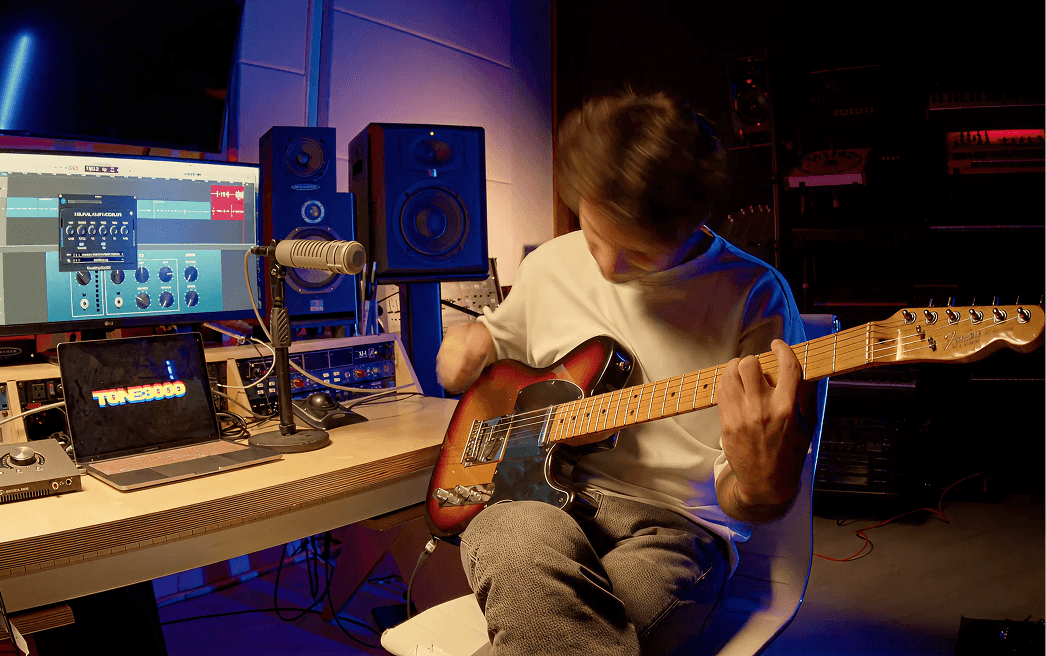
Visit tone3000.com/capture and the website will walk you through capturing your amp, pedal, or signal chain. A2 is the default for all new captures. If you're new to capturing, start with our sweep signal capture guide.
How does training time for A2 compare to A1?
It's comparable on the same hardware.
Do I need to train A2-Full and A2-Lite separately?
No. When you submit a training, TONE3000 creates one A2 model which automatically contains both sizes.
Will my application pick between A2-Full and A2-Lite automatically?
Yes. The application or device will often handle this automatically based on its CPU budget. Some applications will also let you choose.
What about devices that use "NAM-to-X" conversion?
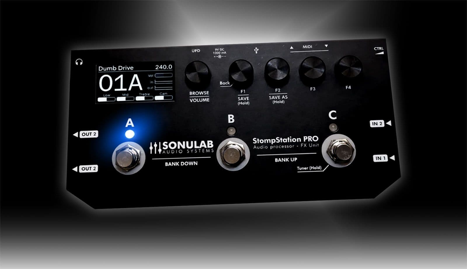
Some companies, including Hotone, Sonicake, Sonulab, Valeton, and NUX, convert NAM A1 models into proprietary formats to run on their chips. Those distilled models are not real NAM models, and they don't have the same sound quality or accuracy.
This is one of the reasons we built A2. A2-Lite is efficient enough to run natively on multi-fx pedals with budget chips, so there's no need for conversion anymore. If your hardware or software maker is still converting NAM files, you can request that they support NAM natively and let them know about A2 and the TONE3000 API :)
Should I separate A1, A2 and Custom architecture files into individual packs?
No. Please don’t do that. Each tone pack on TONE3000 supports all architectures, including A2, A1, and custom architectures in the same pack. The host application or device will load whichever it supports.
Are captures created through dry/wet training compatible with A2?
Yes. The wet-dry training method works the same way with A2 as it did with A1. If you've been capturing your gear using the dry/wet method, nothing about your workflow changes.
For Builders and Integrators
How do I add A2 support to my product?
It depends on the platform.
- Software (plugins and apps): update to NeuralAmpModelerCore (github.com/sdatkinson/NeuralAmpModelerCore) v0.5.2 or later. That's the C++ inference engine, and v0.5.2 is the release that adds A2 support. The A2 fast path is enabled by default via the CMake option
NAM_ENABLE_A2_FAST, which routes A2-shaped models to hand-optimized inference for lower CPU. - Embedded hardware: a C++ engine usually isn't the right fit, so we open-sourced the TONE3000 embedded guide (github.com/tone-3000/nam-pedal): a dependency-free C-engine reference that demos A2 running on the Daisy Seed.
If you want to give your users the ability to browse and load NAM captures and IRs from our constantly expanding library directly within your products, you can integrate the TONE3000 API. For questions or onboarding, reach out at support@tone3000.com.
Does the TONE3000 API support A2?
Yes. Right now, you'll need to specifically request A2 in your API calls. We’ve left A1 as the default for backwards compatibility for now, but A2 will become the default in a future release. For documentation and onboarding details, visit tone3000.com/api.
Should I use the .namb binary format on embedded?
Yes. The .namb format is a compact binary representation of a NAM model designed for embedded use, developed during TONE3000's Daisy Seed work. A companion app converts standard NAM models into .namb for transfer to the device over USB or Bluetooth, with no quality loss. For details, see our Running NAM on Embedded Hardware blog post.
The Technical Deep Dive
Is A2 still a WaveNet?
Only in spirit. A2 is a stack of WaveNet-like modules and keeps the features that make WaveNet recognizable (dilated causal convolutions with residual and skip connections), but almost everything else departs from the model in van den Oord et al. (2016)
The biggest difference is that A2 is feedforward and deterministic rather than generative. Textbook WaveNet is autoregressive, predicting a probability distribution for each sample from all the previous ones and generating audio sequentially. A2 instead maps input audio to output audio in a single pass, this makes real-time amp modeling possible. The output itself also differs. WaveNet emits a 256-way categorical distribution over µ-law-quantized samples and trains to maximize log-likelihood, whereas A2 outputs the audio sample directly and trains on a regression loss (MSE plus MRSTFT).
WaveNet's signature gated activation, a tanh multiplied by a sigmoid, is gone entirely. A2 uses a single ungated LeakyReLU in its place. The dilation schedule is also reworked. WaveNet doubles its dilations (1, 2, 4, … 512) and repeats the pattern. A2 uses a hand-tuned, non-doubling schedule spread across three dilation stacks that includes a degridding step. Finally, A2 changes the convolutions themselves. WaveNet's dilated convolutions are typically filter-size 2, feeding 1×1 convolutions into a softmax; A2 mixes kernel sizes within a single layer array and ends in a new convolutional head.
What changed in the architecture?
The biggest single change is the activation function. A2 uses a leaky ReLU instead of the hyperbolic tangent (Tanh) used in A1. This turned out to be the key that unlocked better accuracy at a lower CPU cost.
Tanh is a genuinely good activation function. A1 models that use it are accurate, both in sample-wise error and in frequency-domain behavior. The catch is that Tanh is expensive to compute on very small networks. Swapping in leaky ReLU freed up enough headroom to grow the network. At the same CPU usage, a larger network with a lighter activation came out more accurate. This result held across many experiments and became a core ingredient of A2.
The other major changes:
- A convolutional head. A1's head worked per-sample, like a waveshaper. A2's spans a window of samples, making it a more expressive mixer.
- Mixed kernel sizes in one layer array. The original WaveNet and A1 gave each dilation stack its own array with a single kernel size. A2 mixes kernel sizes within one array, which enables more flexible tuning and cuts inference-time CPU.
- Refined dilation patterns. Tuned via HPO for optimal connectivity, even receptive-field coverage and a degridding step to stop the build-up behind ringing.
- A larger receptive field. About 6,350 samples (~132 ms at 48 kHz), up from ~4,100 in A1-Standard (~85 ms).
- Slimmable training. Enables a single model to run at A2-Full or A2-Lite size.
How does A2 reduce high-frequency artifacts?
Historically, small WaveNet-based models produced two distinct artifacts, commonly referred to as aliasing and ring. A2 reduces both.
Aliasing-like artifacts. Classical aliasing comes from digital sampling: when a signal contains frequencies above the Nyquist limit (half the sampling rate), they fold back into the audible band as spurious, inharmonic tones. The errors in neural models resemble that same sound, and are often blamed on the network's nonlinear activations generating harmonics above Nyquist. A2's head convolves over a window of samples, mixing the skip outputs across time, rather than instant-by-instant. That extra context lets it shape the high-frequency response directly, smoothing artifacts. We used chirp evals and spectrograms to track the improvement.
Aliasing-like Artifacts
The same sine sweep run through the old and new model designs, compared against the recording.
Ring artifacts: A spectral ringing builds up when harmonics (especially odd ones) over-accumulate through the network, and the effect is most audible on high-gain amps. We ran extensive HPO on the dilation connectivity with two aims: covering the receptive field evenly, and keeping odd harmonics from over-accumulating. Even coverage matters because stacked dilated convolutions are prone to gridding: gaps where some input positions are never sampled. On top of that we added a pair of wide-kernel layers between two dilation stacks that re-mix the gaps the stacks leave behind, a degridding step that smooths and resets the model's effective receptive field. It's only possible because A2 allows mixed kernel sizes in one layer array.
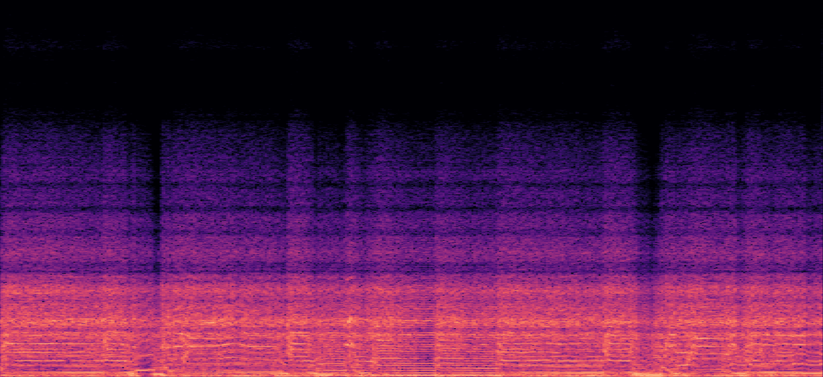
Spectral Ring Artifacts
White noise bursts run through each model variant. Pay attention to the ringing artifact around 10 kHz.
How was the training recipe developed?
We ran thousands of HPO runs that searched learning-rate schedulers, loss functions, and weights (most of the new losses were thrown out), landing on a main loss of MSE (mean squared error) plus a small multi-resolution STFT (MRSTFT) term to keep the frequency-domain behavior honest. ESR is tracked as the validation loss for picking the best checkpoint.
The A2 recipe also normalizes training data to a fixed -18 dB RMS reference, the level the HPO was tuned for, and folds the rescale back into the head scale. Output stays correctly leveled with no extra inference step, and every tone trains under the same conditions, which keeps results consistent and optimal.
What is "slimmable NAM" and how does it work?
Slimmable NAM is a training technique developed by Steve Atkinson that lets a single trained network run at multiple widths, so one model produces multiple size variants without retraining. A2-Full and A2-Lite are two "slim points" of the same model. In the final architecture, an 8-channel network (A2-Full) and a 3-channel network (A2-Lite), are packed into a single file.
You can compare this to rendering an impulse response, where you can use a 512-, 1024-, or 2048-sample truncation depending on the hardware without re-recording anything. Slimmable NAM gives you a similar quality-vs-cost dial for neural amp models, though it works by adjusting the network's effective size rather than truncating a fixed-length response.
Steve's paper, Slimmable NAM: Neural Amp Models with adjustable runtime computational cost, was accepted to the NeurIPS 2025 workshop on AI for Music: arxiv.org/abs/2511.07470
What is "packed" training and how does it work?
Packed training is a variant of slimmable used in the A2 recipe: one training run produces multiple sizes that ship as a single model, and the device runs whichever fits its budget. The difference from the original approach is in how the sizes share weights.
In the original slimmable approach, the smaller size is a channel sub-slice of the larger one. Sharing forces those weights to serve both sizes at once, which costs some accuracy. The packed variant gives each size its own block of weights inside the same model: the sizes train together, but the layers are block-structured so each size only reads and writes its own channels, and a mask holds the cross-size weights at exactly zero after every optimizer step. Because the sizes no longer share parameters, neither has to compromise for the other.
What else did the team explore?
A lot. Here’s a short list:
- Alternative base architectures, including LSTM and a bespoke Hammerstein-Wiener model.
- A half-dozen activation functions, before leaky ReLU won on the accuracy-per-CPU trade-off.
- FiLM (feature-wise linear modulation) layers, which steer scale-and-shift operations inside the network from the conditioning input.
- Alternative head designs, including 1×1 head projections and various nonlinear head mixins.
- Grouped convolution, which splits a layer's channels into independent groups to cut compute.
- Bottlenecks in the WaveNet layers, where channel counts shrink or grow before the activation.
- A conditioning module that moved part of the network "up" so its output fed directly into every layer.
- Auxiliary loss functions, including a spectral-band loss that penalized energy in problem frequency bands, and ESR as a training term.
- Training-recipe experiments: EMA weight averaging, random window offsets as augmentation, adding chirps to the training data, and a range of learning-rate schedulers.
- Aggressive model quantization and distillation to push embedded performance even further.
Simplicity won when results were close. The team ran well over ten thousand trainings in hyperparameter optimization (HPO) experiments, varying kernel sizes, dilation patterns, channel counts, activations, and architectural choices to map out the trade-offs, with GPUs running day and night.
What evaluation metrics were used?
Four primary error metrics:
- ESR (error-signal ratio): a normalized version of mean squared error. Measures how closely the model's output matches the reference sample by sample, factored out from absolute level.
- MAE (mean absolute error): measures the same kind of sample-wise error with a different statistical sensitivity.
- LOG_MEL: measures how closely the model's mel-spectrogram matches the reference, capturing frequency-domain accuracy in a way that lines up with how humans hear.
- MRSTFT (multi-resolution short-time Fourier transform): measures spectral accuracy at multiple time-frequency resolutions, catching both transient detail and longer-term frequency content.
Each model is scored on all four metrics across the evaluation set. Those scores drive head-to-head comparisons between models, which feed Bayesian Elo ratings. Models that win their matchups more earn higher ratings, giving one overall number that summarizes performance across the whole set.
What was in the evaluation set?
The evaluation set included guitar and bass amps, pedals, amp and pedal chains, outboard studio gear, and full rigs of amps and cabs. We incorporated a wide variety of tones, from sparkling Fender cleans, to a vintage Neve 1073, to a dimed Mesa Boogie Dual Rectifier, with an octave fuzz to stress-test extreme distortion. 39 distinct tones in total.
How was the listening test run?
We conducted a formal, large-scale blind listening test using the MUSHRA methodology. MUSHRA ("Multiple Stimuli with Hidden Reference and Anchor") is the gold standard for evaluating percieved audio quality, used by broadcasters like the BBC and EBU.
Over 1,000 participants submitted more than 100,000 ratings, which might be the largest tone study ever done. In each trial a participant heard the real recorded gear first as a reference, then rated several subsequent versions of that same tone, modeled with A2-Full, A2-Lite, A1-Standard, A1-Nano, Neural DSP’s Neural Capture V2, IK Multimedia’s ToneX, and Line 6’s Proxy, without knowing which was which. Participants scored each model on how closely it matched the original recording, using a 0–100 scale.
Per MUSHRA methodology, two of the clips in each trial were quality controls. One was a duplicate of the original, a ‘hidden reference’ meant to score highly, and the other was designed to sound worse, a ‘low-passed anchor’ meant to score low. This allows for post-screening to remove bad data; in our case, we dropped the results from participants who rated the hidden reference too low or the low-passed anchor too high, so that they didn’t skew the result.
Both the test code and the raw ratings are open source:
- Test code: github.com/tone-3000/t3k-mushra
- Raw data: github.com/tone-3000/a2-mushra-data
Tests were conducted in March 2026 using the latest modelers from Neural DSP, IK Multimedia ToneX, and Line 6 Proxy.
What's this Lord of the Rings business?
During development, the team explored so many candidate architectures that we needed a way to keep track of them. Over 42 made it to the production-candidate stage, and the team started naming them after characters from The Lord of the Rings. The final call was between Boromir and Legolas. In an ending no one saw coming, Boromir won.
What's the difference between NAM and A2?
NAM is an open-source framework for neural amp modeling. It contains the tools to train a neural model from a recording and run it in real time. NAM can train and run a range of architectures, from a simple linear model to ConvNets, LSTMs, and WaveNets, each with countless configurations.
A2 is a specific architecture created with NAM. It’s designed to be an open standard that hardware manufacturers and software developers will adopt.
How does A2 run so efficiently?
A2's efficiency comes from two places. The first is the architecture itself, covered above. The second is the inference engines that run the models. We rebuilt NAM inference on two open-source fronts, a hand-optimized fast path in the C++ core for plugins and apps, and a dependency-free C engine for embedded hardware.
The fast path lives in NeuralAmpModelerCore and is on by default (NAM_ENABLE_A2_FAST). The hot operation in a WaveNet is the 1×1 convolution that mixes channels. It's really just a small matrix multiply, run once per layer per block. General-purpose math libraries are tuned for big matrices and waste time on setup and temporary allocations at NAM's tiny sizes, so the fast path swaps in fully unrolled, register-resident kernels sized to A2's channel counts. On an Apple M5, that takes A2-Lite from a 50x real-time factor on the original Eigen path to 316x. That's roughly 6x faster on the same model, from inference engineering alone.
Desktop Inference Speed
How fast A2-Lite runs on a modern desktop CPU, and how much headroom is left for the rest of your signal chain.
Embedded is a harder problem. A C++ engine that leans on a general math library is a poor fit for a microcontroller with a scalar FPU and a few hundred KB of RAM. The dependency-free C engine we built and published for embedded targets fixes that. On the Daisy Seed (ARM Cortex-M7 at 480 MHz, the chip class behind many DSP pedals), A2-Lite clears real time on both the fast path and the purpose-built engine.
Embedded Inference Speed
Whether A2-Lite can run in real time directly on resource-constrained embedded hardware.
Under the hood, the embedded wins are a stack of low-level tricks, each kept only because a microbenchmark said it paid off on the Cortex-M7. Those include hand-written unrolled matrix multiplies in place of a general library (the single biggest win), fused layers that keep intermediate values in registers, lookup-table activations instead of exp, weights pinned in tightly-coupled memory while the ring buffers stay in cached SRAM, and power-of-2 ring buffers that give constant, spike-free per-block timing. The full per-operation breakdown, including the cases where the general library actually won, is in João's writeup, the embedded reference engine, and the C++ core.
What's next?
We're proud of A2 and excited to hear what you think.
As a next step, we're open-sourcing our evaluation and listening-test code along with the raw data. We want this work to be peer-reviewed, stress-tested, and replicated. If you can reproduce our results, or poke holes in our methods, we want to hear from you.
A lot of what makes an amp feel right happens under your hands in real time, and that's something a recorded evaluation can't fully capture. So we're especially eager to hear how these models feel to actually play, and to see new evaluation methods that build on what we've shared.
Go play!
Related Blog Posts

Trending Tones


NEW TO TONE3000?
Discover hyper-realistic digital models of iconic gear, including the Fender Twin Reverb, Vox AC30, Marshall JCM 800, and thousands more. Getting started is easy—and free!